Vector Database Indexes
Introduction to Vector Indexing
When building applications with Large Language Models (LLMs), RAG, or semantic search systems, high-dimensional vector embeddings (typically ranging from 256 to 1536+ dimensions) are generated. Comparing a query vector against millions of stored vectors using an exact brute-force search requires O(N) time complexity. This creates a massive scaling bottleneck, grinding production systems to a halt.
Vector database indexes solve this by organizing high-dimensional vector spaces so you can perform Approximate Nearest Neighbor (ANN) searches. Instead of checking every single record, these indexes trade a tiny, controllable fraction of accuracy (recall) for massive, orders-of-magnitude increases in search speed (O(log N) or O(1) amortized time).
1. Flat Index (No Index / Brute Force)
It isn't actually an "approximate" index. It stores vectors exactly as they are without any structural modification, partitioning, or clustering.
How it is Implemented
- Storage: Vectors are stored as continuous, sequential arrays of floating-point numbers (
FP32,FP16) in memory or on disk. - Search Mechanism: When a query arrives, the system calculates the exact distance (e.g., Cosine similarity, Euclidean distance, or Dot Product) between the query vector and every single vector in the entire database.
Problem it Solves
- Eliminate information loss and recall degradation.
- If you Need to find exact mathematically nearest neighbors.
Pros & Cons
- Pros:
100%perfect recall (perfect accuracy).- Zero build/training time.
- Inserting new vectors is instantaneous (
O(1)).
- Cons:
- Search time scales linearly with data size (
O(N)). - Unusable for production apps with thousands or millions of vectors.
- Extremely CPU/GPU intensive during queries.
- Search time scales linearly with data size (
Search Speed & Latency Impact
- Access Speed Complexity:
O(N * D), whereNis the number of vectors andDis the dimensionality. - Real-world feel: Latency scales linearly with vectror size
Use Cases & Design Patterns
- Small Datasets: Collections with fewer than 10,000 vectors.
- Ground Truth Evaluation: Used as a golden baseline benchmark to evaluate the accuracy (recall) of other ANN indexes.
2. Inverted File Index (IVF)
IVF is a space-partitioning index designed to narrow down the search space by grouping similar vectors together into local buckets before running queries.
How it is Implemented
- Training Phase (K-Means): It uses the K-Means Clustering algo to partition the high-dimensional vector space into
Kdistinct clusters. Each cluster is anchored by a central point called a centroid. - Inverted List Structural Pattern: It maps each unique centroid ID to an inverted list containing the IDs and values of all vectors belonging to that specific cluster.
- Search Mechanism: When a query vector arrives, the system first compares it against the
Kcentroids to find the closest ones. It then only searches the vectors inside those specific closest clusters, entirely skipping the rest of the database.
Deeper Dive: K-Means Clustering Core Mechanics
- Initialization: The database selects
Krandom vectors from the dataset to act as the initial centroids. - Assignment Phase: The algorithm iterates through every single vector in the training set, calculates its distance to all
Kcentroids, and assigns the vector to its mathematically nearest centroid. - Update Phase: For each of the
Kclusters, the algorithm calculates the mean vector of all data points currently assigned to it. This new mean vector becomes the updated centroid. - Convergence: Steps 2 and 3 repeat iteratively until the centroids stop moving significantly (or a maximum iteration threshold is hit).
This process carves the high-dimensional space into geometric regions called Voronoi cells. Every point inside a specific Voronoi cell is closer to that cell's centroid than to any other centroid in the database.
Deeper Dive: The nprobe Parameter (The Speed vs. Accuracy Knob)
nprobe is a dynamic, query-time configuration parameter used exclusively with IVF indexes. It dictates how many of the nearest clusters (Voronoi cells) the database will open up and search during a query.
- The Edge Effect Problem: If your query vector lands near the boundary/edge of a cluster, its true nearest neighbors might actually reside just across the border in an adjacent cluster.
- If
nprobe = 1: The database looks only inside the single closest cluster. If your true nearest neighbor is across the border, you miss it, resulting in lower recall. - If
nprobe = K: The database searches all clusters, transforming the IVF index right back into a slow, brute-force Flat index. - The Trade-off: Low
nprobe(e.g., 1 to 5) gives blazing-fast latency but lower recall accuracy. Highnprobe(e.g., 32 to 128+) gives high recall accuracy but latency increases linearly with the number of vectors checked.


- How Search is performed
                    [ Query Vector ]
                              │
               ┌──────────────┴──────────────┐
               ▼                             ▼
     [ Compute Distances to All Centroids in Registry ]
               │
               ▼
     [ Rank Centroids by Distance: C2 (Closest), C1 (2nd Closest), C3 (Far) ]
               │
      ┌────────┴────────┬───────────────────┐
      │ (If nprobe=1)   │ (If nprobe=2)     │ (If nprobe=3)
      ▼                 ▼                   ▼
[ Search List C2 ]   [ Search Lists ]    [ Search Lists ]
                     [   C2 and C1  ]    [ C2, C1, and C3]
Problem it Solves
It drastically cuts down the number of vector comparisons from N to a tiny fraction of N by eliminating irrelevant geometric regions early in the query lifecycle.
Pros & Cons
- Pros:
- Significantly reduces search latency compared to Flat indexes.
- Low memory footprint compared to graph-based structures.
- Cons:
- Requires a slow, computationally intensive "training/build" step.
- If your data distribution shifts significantly over time (data drift), you must completely re-index.
- Vulnerable to lower recall if
nprobeisn't carefully tuned.
Search Speed & Latency Impact
- Access Speed Complexity: Reduces search complexity down to
O(K + nprobe*(N/K)). - Real-world feel: Sub-10ms search times even on millions of rows, depending on your chosen trade-off balance.
Use Cases & Design Patterns
- Memory-Constrained Production Systems: When you have millions of vectors but want to keep the active index memory footprint small and low-cost.
- Partitioned Multitenancy: Excellent when you can cluster data naturally by customer ID or data category, pairing structural metadata filtering with IVF lists.
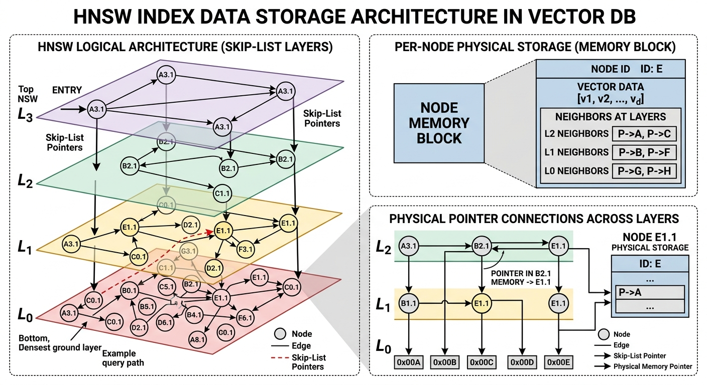
3. Hierarchical Navigable Small World (HNSW)
- HNSW is currently the gold standard for high-performance production vector databases.
- Used by default in tools like Pinecone, Milvus, Weaviate, Qdrant, and pgvector.
- It is a graph-based index.
How it is Implemented & Inner Workings
-
It builds an explicit, multi-layered graph data structure.
-
It borrows its architectural philosophy from the Skip List, mapping it to a graph representation to solve the "local minima" problem (where a graph search gets stuck in a cluster of nodes because it cannot see the bigger geometric picture).
-
Multi-layer Graph Architecture:
- Layer 0 (Bottom Layer): Contains every single vector in the database. The graph connections here are short-range, dense, and highly detailed.
- Upper Layers (Layer 1 to Layer
L): Contain an exponentially decreasing subset of vectors. The links here span massive structural distances across the vector space, creating global shortcuts. The probability of an inserted element scaling to a higher layer decays exponentially according to a scaling factor (1/\ln(M)).
-
The Routing Mechanism (The Search):
- The search begins at a predefined entry point node in the top-most layer.
- It performs a greedy search: it checks the neighbors of the current node and moves to whichever neighbor is closest to the query vector.
- When it reaches a node where none of its neighbors are closer to the query than the current node itself (a local minimum for that specific layer), it drops down to the corresponding node in the next layer below.
- It repeats this process, using the entry point from the layer above to bootstrap the new local search.
- Once it reaches Layer 0, it executes a granular nearest-neighbor search using a priority queue (nearest points)(bounded by a configuration parameter called
efSearch) to return the final top-K results.

Problem it Solves
It solves the trade-off bottleneck between blazing-fast speed and exceptionally high recall (often 95-99% accuracy) on massive-scale datasets.
Pros & Cons
- Pros:
- Incredible search speeds with logarithmic scaling (
O(log N)). - Highest recall accuracy among all approximate indexes.
- Supports incremental, real-time updates seamlessly (inserting or deleting nodes) without needing to rebuild the entire graph structure.
- Incredible search speeds with logarithmic scaling (
- Cons:
- Massive memory consumption. The explicit graph links and pointers require substantial RAM overhead on top of the vectors themselves.
- Building the graph is computationally heavy and takes significantly longer to train/build compared to other formats.
Search Speed & Latency Impact
- Access Speed Complexity: True logarithmic scale,
O(log N). - Real-world feel: Ultra-low latency, typically between 1ms to 5ms for queries over millions of vectors.
Use Cases & Design Patterns
- High-Performance Production RAG: Enterprise search engines, real-time chatbots, and high-throughput recommendation systems where latency budgets are razor-thin (e.g., sub-20ms SLAs).
- Dynamic Data Streams: Applications where data is constantly being inserted, updated, or deleted in real time without downtime.
4. Product Quantization (PQ) & Scalar Quantization (SQ)
Quantization indexes are structural compression techniques. While frequently paired with other indexing techniques (like IVF or HNSW), they function as distinct index strategies focused primarily on memory optimization.
How they are Implemented
- Scalar Quantization (SQ): Converts the underlying data type of the vector dimensions. For example,
SQ8(an algo to covert- not readed more)compresses 32-bit floating-point numbers (FP32) down to 8-bit signed/unsigned integers (INT8). It shifts the precision window uniformly. - Product Quantization (PQ): A more advanced, lossy compression strategy:
- It splits a high-dimensional vector of size
DintoMsmaller, independent sub-vectors. - Each sub-vector space is clustered using
K-Meansto find local centroids. - Each original sub-vector is then replaced by a compact, short byte-sized code (typically 1 byte) representing the ID of its nearest sub-cluster centroid.
- It splits a high-dimensional vector of size
- Search Mechanism: Distance calculations are performed directly on these compressed codes using Asymmetric Distance Computation (ADC). Instead of decompressing vectors back to floats, the engine constructs a fast lookup table of distances from the query vector to the sub-centroids, running simple additions over the bytes.
Problem it Solves
The RAM Cost Problem. Storing millions of high-dimensional FP32 vectors completely in RAM is prohibitively expensive. Quantization shrinks the memory footprint by up to 70% to 95%, allowing lean infrastructure footprints.
Pros & Cons
- Pros:
- Massive memory savings (e.g., a 100GB vector dataset can be compressed down to less than 10GB).
- Drastically reduces hardware infrastructure costs.
- Can accelerate raw CPU throughput because smaller byte streams fit cleanly into CPU L1/L2 caches.
- Cons:
- Introduces structural approximation errors during compression, which directly degrades overall recall/accuracy.
- High training overhead to establish the initial quantization codebooks.
Search Speed & Latency Impact
- Access Speed: Highly dependent on the base index layout it is attached to, but the direct ADC byte-lookups are exceptionally fast, keeping latency comparable to or slightly faster than uncompressed variations at the cost of precision.
Use Cases & Design Patterns
- Billion-Scale Vector Search: When you are managing hundreds of millions or billions of items and hosting them purely in-memory using raw floats would cost thousands of dollars a month in cloud infrastructure bills.
- Hybrid Storage Patterns (Warm/Cold Storage): Storing compressed PQ codes in memory for initial fast filtering, then fetching the raw vectors from disk to recalculate exact scores for the top candidates.
5. Locality-Sensitive Hashing (LSH)
LSH is an algorithmic approach to partitioning vector space using specialized hashing functions that intentionally maximize hash collisions for nearby points.
How it is Implemented
- Hashing Functions: It passes vectors through a series of hashing functions designed so that vectors close to each other in high-dimensional space have a highly elevated probability of hashing into the same unique "bucket ID."
- Search Mechanism: The incoming query vector is hashed using the exact same functions. The database looks inside that specific hash bucket and evaluates only the vectors residing there, treating the bucket as the candidate pool.
Problem it Solves
It transforms a complex, high-dimensional geometric distance calculation into a straightforward, fast hash table key lookup problem.
Pros & Cons
- Pros:
- Highly scalable and mathematically predictable.
- Simple to implement on traditional distributed map-reduce architectures or standard key-value databases.
- Cons:
- Suffers from lower recall accuracy in very high-dimensional spaces compared to modern graph approaches like HNSW.
- Can create highly uneven bucket distributions (skewed data distributions cause system hot spots).
Search Speed & Latency Impact
- Access Speed Complexity:
O(K), whereKis the number of hash tables/lookups, independent ofNunder ideal uniform data distributions. - Real-world feel: Fast, predictable lookups, but requires massive tuning of hash functions to prevent accuracy drops.
Use Cases & Design Patterns
- Near-Duplicate Detection: Identifying copyright infringements, duplicate web pages in search crawlers, or matching audio fingerprints (e.g., Shazam-like systems) where structural similarity matters more than nuanced semantic context.
6. Advanced Composition: Combining HNSW with Quantization (PQ/SQ)
In modern enterprise systems, engineers rarely use these indexes in pure isolation. Instead, they leverage composite indexing patterns to get the best of both worlds: the speed/accuracy of graphs with the lean footprint of compression.
An uncompressed HNSW index requires keeping the raw FP32 vectors plus the extensive graph edge lists entirely in RAM. For a 768-dimensional embedding model, 1 million vectors can take up over 4–5 GB of RAM. At scale, this becomes unsustainably expensive.
Modern vector engines solve this using two primary composite patterns:
Pattern A: SQ8 + HNSW (The Industry Standard Balanced Choice)
The database applies Scalar Quantization to reduce the vector data type from 32-bit floats (FP32) to 8-bit integers (INT8) before threading them into the HNSW graph.
- How it works: The HNSW graph structure remains exactly the same, but the vector data stored at each node is converted to
INT8. When calculating distances along the graph during a search, the engine uses fast integer math or unquantizes the values on the fly. - Memory Savings: Cuts vector storage footprint by roughly 75% (from 4 bytes per dimension to 1 byte).
- Accuracy Loss: Negligible. You typically experience less than a 1% drop in recall.
Pattern B: PQ + HNSW (Max Compression Choice)
The database applies Product Quantization to divide vectors into chunks and assign them centroid IDs (codes) before building the HNSW graph layout.
- How it works: Distances between graph nodes during routing are calculated using Asymmetric Distance Computation (ADC). Instead of calculating geometric distances using floats, the engine performs lightning-fast array lookups against a precomputed PQ distance table.
- Memory Savings: Massive. Can compress data up to 90% to 95%, allowing huge datasets to fit on a single machine.
- Accuracy Loss: Noticeable. Quantization artifacts can distort graph routing paths, leading to a 5% to 15% drop in recall.
Production Design Pattern: Rescoring / Reranking
To mitigate the accuracy loss of HNSW+PQ, modern databases implement a multi-tiered storage pattern:
- The engine uses the HNSW+PQ index in-memory to quickly fetch the top 100 approximate candidates.
- It then reads the raw, uncompressed
FP32vectors from persistent disk storage (like an NVMe SSD) for just those 100 candidate IDs. - It performs an exact mathematical re-ranking on those 100 records, returning a highly accurate top 10 to the user. This keeps RAM usage incredibly low while maintaining pristine recall.
7. Comparative Reference Matrix
| Index Type | Search Complexity | Memory Footprint | Build/Train Speed | Recall Accuracy | Dynamic Updates? |
|---|---|---|---|---|---|
| Flat | O(N * D) | Low (Raw data only) | Instant (O(1)) | Perfect (100%) | Yes (Native) |
| IVF | O(K + nprobe * (N/K)) | Low | Medium (K-Means) | Medium-High | Hard (Needs Re-training) |
| HNSW | O(log N) | Very High | Slow | Very High (95-99%) | Yes (Native) |
| PQ / SQ | Base index dependent | Extremely Low | Slow (Quantization) | Medium | Hard (Requires re-quantizing) |
| LSH | O(K) | Medium | Fast | Low-Medium | Yes (Native) |